louis meunier

calculus

top

On this page:

Viviani's curve with the TNB frame

Viviani’s curve describes the intersection of a sphere and cylinder, specifically $$(x-r)^2+y^2=r^2, \quad x^2+y^2+z^2=4r^2.$$ The intersection curve can be parametrized $$x = r(1+\cos t)$$ $$y= r\sin t$$ $$z=2r\sin(\frac{t}{2})$$

begin
    using Plots

    r = 10
    x(t) = r*(1+cos(t))
    y(t) = r*sin(t)
    z(t) = 2*r*sin(0.5*t)
    R(t) = [x(t), y(t), z(t)]
    t_range = range(-2π, 2π, length=100)

    tnb_anim = @animate for t_at in t_range
        plot3d(x.(t_range), y.(t_range), z.(t_range), legend=false, aspect_ratio=:equal,
        xlims=(-5,25),
        ylims=(-11,11),
        zlims=(-21,21),
        camera=(30, 15),
        color=RGBA(241/255,90/255,34/255,0.5),
        linewidth=5,
        )

        plot3d!([R(t_at)[1]], [R(t_at)[2]], [R(t_at)[3]], color=:black, marker=:circle, markersize=3, label="t = $t_at")

        # T
        T_hat = R'(t_at)/norm(R'(t_at))
        arrow!(R(t_at), 2.5*T_hat, color=:red, label="T", linewidth=3, aspect_ratio=:equal)

        # N
        N_hat = cross(R'(t_at), cross(R''(t_at), R'(t_at)))/(norm(R'(t_at))*norm(cross(R''(t_at), R'(t_at))))
        arrow!(R(t_at), 2.5*N_hat, color=:green, label="N", linewidth=3, aspect_ratio=:equal)

        # B
        B_hat = cross(T_hat,N_hat)
        arrow!(R(t_at), 2.5*B_hat, color=:blue, label="B", linewidth=3, aspect_ratio=:equal)
    end
    gif(tnb_anim, "tnb.gif", fps=20)
end

Visualizing a parametrically defined curve orthogonal to a surface

The curve $F$ is defined parametrically by $x(t) = \frac{2(t^3+2)}{3}$, $y(t) = 2t^2$, and $z(t) = 3t-2$. The surface $G$ is defined implicitly as $15 = x^2+2y^2+3z^2$. $F$ is perpendicular to $G$ at $P = (2,2,1)$. We can prove this by finding the gradient of the two functions; if the two functions are truly perpendicular at this point, then the gradients should simply by multiples of each other.

$$\nabla \vec{G}(t) = \langle 2t^2, 4t, 3\rangle$$

$$\nabla \vec{F}(x,y,z) = \langle 2x, 4y, 6z\rangle$$

At the point $P$, $t = 1$, so we can find the gradients at $P$:

$$\nabla \vec{G}(1) = \langle 2, 4, 3\rangle$$

$$\nabla \vec{F}(2,2,1) = \langle 4, 8, 6\rangle$$

Clearly, $\nabla \vec{G}(1) = 2\nabla \vec{F}(2,2,1)$, indicating these two gradients are in the same direction, and as such, the curve $F$ is perpendicular to the surface $G$ at $P$. This can be understandably difficult to reason, so the following visualization may help.

# julia
# MATH150 Assignment 5, Problem 9a
begin
using Plots; plotly()
# general "settings"
t_range = range(0.95, stop=1.05, length = 100)
P = [2,2,1]
# F, a curve defined parametrically
x(t) = 2(t^3+2)/3
y(t) = 2t^2
z(t) = 3t-2

F_x_range = x.(t_range)
F_y_range = y.(t_range)
F_z_range = z.(t_range)

plot(F_x_range, F_y_range, F_z_range, color=RGBA(0,0,255,0.5), linewidth=3, label="F", legend=false)

# G
g(x,y) = sqrt((15-x^2-2y^2)/3)
G_x_range = range(1.9, stop=2.1, length = 100)
G_y_range = range(1.9, stop=2.1, length = 100)
# G_z_range = g.(G_x_range, G_y_range)
surface!(G_x_range, G_y_range, g, color=RGBA(255,0,0,0.5), linewidth=3, label="G", legend=true)
# plotting the point of interest
plot!(
    [2],[2],[1],
    marker = (:circle, 1, 0.8, :black),
    label = "P(2,2,1)"
)

# I multiply each vector by a scalar to make them fit within the bounds of the functions
scalar = 0.01
# plot the gradient of G
grad_G_x(t) = 2t^2
grad_G_y(t) = 4t
grad_G_z(t) = 3
# note that t = 1 at P = (2,2,1)
plot!(
    [P[1], P[1]+scalar*grad_G_x(1)],
    [P[2], P[2]+scalar*grad_G_y(1)], 
    [P[3], P[3]+scalar*grad_G_z(1)],
    color=:green,
    linewidth=6,
    label="grad G(2,2,1)"
)

# plot the gradient of F
grad_F_x(x,y,z) = 2x
grad_F_y(x,y,z) = 4y
grad_F_z(x,y,z) = 6z

plot!(
    [2, 2+scalar*grad_F_x(P[1],P[2],P[3])],
    [2, 2+scalar*grad_F_y(P[1],P[2],P[3])], 
    [1, 1+scalar*grad_F_z(P[1],P[2],P[3])],
    color=:orange,
    linewidth=6,
    label="grad F(2,2,1)"
)
end

Newton’s method animation

Newton’s method animated to find the root of a function, $f(x)=x^3-2x^2-x+2$, with an initial estimate of $x = 0.15$.

$$ x_n = x_{n-1} - \frac{f(x_{n-1})}{f'(x_{n-1})} $$

# Julia
begin
    using LaTeXStrings, Plots;
	f(x) = x^3-2x^2-x+2
	g(x) = 3x^2-4x-1

	max_est = 6
	true_value = 1
	z = ones(max_est)
	z[1] = 0.15
	
	for i=2:max_est
		z[i] = z[i-1] - f(z[i-1])/g(z[i-1])
	end

	newtons_methods_animation = @animate for i = 1:max_est
	    plot(
			f,
			-1, 2,
			framestyle=:origin,
			legend=:none,
		)
		plot!(
			[z[i]],
			[0],
			color=:red, marker=:circle, markersize=5,
		)
        if (i > 1)
            est(x) = (
                g(z[i-1])*(x-z[i-1])
                )+f(z[i-1])
            plot!(est)
            plot!(
                [z[i-1], z[i-1]],
                [0, f(z[i-1])],
                color=:pink
            )
            plot!(
                [z[i-1]],
                [0],
                color=:red, 
                marker=:circle, 
                markersize=5,
            )
            annotate!(
                [z[i-1]],
                [-0.2],
                latexstring("x_{", i-1, "}"),
            ) 
        end
        plot!(
            [z[i], z[i]],
            [0, f(z[i])],
            color=:purple
        )
        annotate!(
            [z[i]],
            [0.2],
            latexstring("x_{", i, "}"),
        )
		annotate!(
			1.5,1.5, 
			text(
				latexstring("x_", string(i), " = ", string(round(z[i],digits=3)))
			)
		)
		annotate!(
			1.5, 1, 
			text(
				latexstring("\\% error = ", string(round(100*(abs(true_value - z[i]))/true_value, digits=3)))
			)
		)
		ylims!(-1,2.5)
	end 
	gif(newtons_methods_animation, "tutorial_heatmap_anim.gif", fps = 1)
end

chain rule tree diagrams

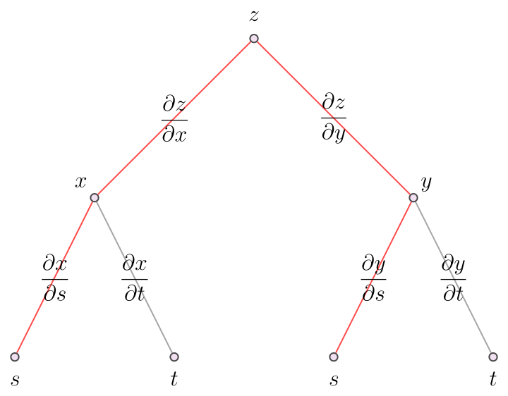
How I make trees to visualize the chain rule of derivatives (in Mathematica). I used the MaTeX package to render the labels as latex, but this could be replace with just normal text strings.

(* mathematica *)
<< MaTeX`
Graph[
 {
  Labeled[1, MaTeX["z", FontSize -> 16]],
  Labeled[2, MaTeX["x", FontSize -> 16]],
  Labeled[3, MaTeX["y", FontSize -> 16]],
  Labeled[4, MaTeX["s", FontSize -> 16]],
  Labeled[5, MaTeX["t", FontSize -> 16]],
  Labeled[6, MaTeX["s", FontSize -> 16]],
  Labeled[7, MaTeX["t", FontSize -> 16]]
  },
 {
  1 <-> 2,
  2 <-> 4,
  1 <-> 3,
  2 <-> 5,
  3 <-> 6,
  3 <-> 7
  },
 EdgeLabels -> {
   1 <-> 2 -> 
    MaTeX["\\frac{\partial z}{\partial x}", FontSize -> 16],
   2 <-> 4 -> 
    MaTeX["\\frac{\partial x}{\partial s}", FontSize -> 16],
   1 <-> 3 -> 
    MaTeX["\\frac{\partial z}{\partial y}", FontSize -> 16],
   2 <-> 5 -> 
    MaTeX["\\frac{\partial x}{\partial t}", FontSize -> 16],
   3 <-> 6 -> 
    MaTeX["\\frac{\partial y}{\partial s}", FontSize -> 16],
   3 <-> 7 -> MaTeX["\\frac{\partial y}{\partial t}", FontSize -> 16]
   },
 GraphLayout -> "LayeredEmbedding",
 EdgeStyle -> {
   1 <-> 2 -> Red,
   2 <-> 4 -> Red,
   1 <-> 3 -> Red,
   2 <-> 5 -> Gray,
   3 <-> 6 -> Red,
   3 <-> 7 -> Gray
   },
 VertexSize -> 0.05,
 VertexStyle -> LightPurple
]

“the shark problem” From the James Stewart Calculus book (pg. 985, no. 2).

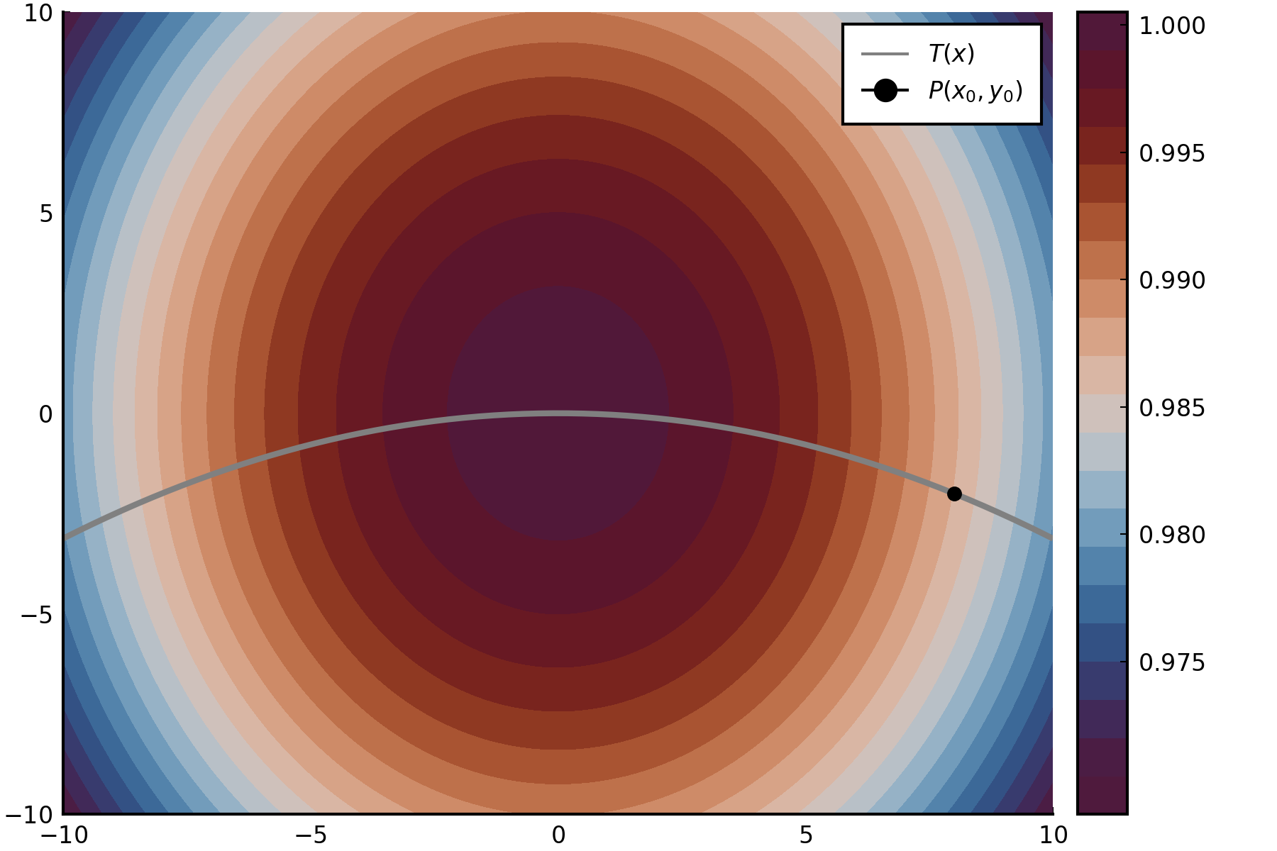
“Marine biologists have determined that when a shark detects the presence of blood in the water, it will swim in the direction in which the concentration of the blood increases most rapidly. Based on certain tests, the concentration of blood (in parts per million) at a point $P(x,y)$ on the surface of seawater is approximated by $$C(x,y) = e^{\frac{-(x^2+2y^2)}{10^4}}$$ where $x$ and $y$ are measured in meters in a rectangular coordinate system with the blood source at the origin."

The graph below represents the situation, where $T(x)$ is the function of the direction that the shark will take given a particular starting point $P(x_0,y_0)$.

begin
    using Plots, LaTeXStrings; pyplot() 
    # initial condition
    x_0 = 8
    y_0 = -2
    # the "concentration of blood" on the surface of the water
    C(x,y) = ℯ^(-(x^2+2y^2)/(10^4))
    x_range = -10:0.1:10
    y_range = -10:0.1:10
    C_range = [C(x,y) for x in x_range, y in y_range]
    contourf(
        x_range,
        y_range,
        C_range, 
        color=:vikO,
        levels=20,
        dpi=300
    )

    t(x) = (y_0/(x_0)^2)*x^2
    t_range = t.(x_range)
    z_path_range = C.(x_range, t_range)
    plot!(
        x_range,
        t_range,
        color=:gray,
        linewidth = 2,
        label=L"T(x)"
    )
    plot!(
        [x_0],
        [y_0],
        color = :black,
        markersize = 4,
        marker = :circle,
        label = L"P(x_0, y_0)"
    )
    xlims!(-10,10)
    ylims!(-10,10)
end

tangent plane of a function of $x$ and $y$

Finding the tangent plane of: $$f(x,y) = 4x^2+4xy+y^2+2x+5y+3$$ at: $$(x_0,y_0,z_0) = (-3,1,27)$$

$$ t(x,y) - z_0 = \frac{\partial f}{\partial x}(x,y)(x-x_0) + \frac{\partial f}{\partial y}(x,y)(y-y_0) $$ $$t(x,y) = -18x-5y-22$$

# Julia
begin
	using  Plots;
	
	plotly()

	transparent_red = RGBA(200/255,60/255,60/255,200/255)
	transparent_gray = RGBA(30/255,30/255,30/255,230/255)
	
	abc(x,y) = 4x^2+4x*y+y^2+2x+5y+3

	x_range = range(-10,stop=10,length=100)
	
	surface(
		x_range,
		x_range,
		abc,
		color = transparent_red,
		label = "f(x,y)",
		legend = :none
	)
	
	surface!(
		x_range,
		x_range,
		(x,y) -> -18x-5y-22,
		color = transparent_gray,
		label = "t(x,y)"
	)
	
	plot!(
		[-3], [1], [27], 
		color=:blue, 
		marker=:circle, 
		markersize=2, 
		label = "point"
	)
end

tangent plane of a parametric function

Given a sphere defined parametrically as a function $F(x,y,z)$:

$$x = r\cos\theta\sin\phi$$ $$y = r\cos\theta\cos\phi$$ $$z = r\sin\theta$$

where $r$ is the radius of the sphere, $\theta$ is the polar angle (along the $x-z$ plane), and $\phi$ is the azimuthal angle (along the $x-y$ plane). Since $x$, $y$, and $z$ are all functions of $\theta$ and $\phi$, we can define a vector function $G(\theta,\phi)$:

$$G(\theta,\phi) = \langle x(\theta,\phi), y(\theta,\phi), z(\theta,\phi)\rangle$$ $$=\langle r\cos\theta\sin\phi,\cos\theta\cos\phi,r\sin\theta \rangle$$

Taking the derivative of $G$ with respect to $\theta$ and $\phi$:

$$G_{\theta} = \langle -r\sin\theta\sin\phi, -r\sin\theta\cos\phi, r\cos\theta\rangle$$ $$G_{\phi} = \langle r\cos\theta\cos\phi, -r\cos\theta\sin\phi, 0\rangle$$

These functions represent vectors, clearly, and are tangent to the sphere at some point, say, $P(\theta_0, \phi_0)$. Intuitively, we can find the equation for a normal line to the sphere at $P$ by taking the cross product of $G_{\theta}$ and $G_{\phi}$, as this yields the vector normal to both:

$$G_{\perp} = G_{\theta}\times G_{\phi} = \langle r^2 \cos \theta \sin \theta \sin \phi, -r^2 \cos \theta \sin \theta \cos \phi, -r^2 \cos^2 \theta\rangle$$

The tangent plane to the sphere at $P$, intuitively, is also normal to this vector. Thus, we can find an equation for the plane by taking the dot product of the normal vector with the corresponding $(x_0,y_0,z_0)$ to $P$:

$$0 = G_{\perp} \cdot \langle x-x_0, y-y_0, z-z_0 \rangle$$

$$0 = r^2 \cos \theta \sin \theta \sin \phi (x-x_0) -r^2 \cos \theta \sin \theta \cos \phi (y-y_0) -r^2 \cos^2 \theta (z-z_0) $$

Rearranging for $z$ as a function of $x$ and $y$:

$$z = \frac{r^2 \cos \theta \sin \theta \sin \phi (x-x_0) -r^2 \cos \theta \sin \theta \cos \phi (y-y_0)}{r^2 \cos^2 \theta} -z_0 $$

For instance, take $P = (x,y,z) = (1,1,\sqrt{2})$. The tangent plane at this point, simplified:

$$z = \frac{1}{2}x + \frac{1}{2}y - \sqrt{2}$$

# Julia
begin
    using Plots; plotly()

    # radius of the sphere
    r = 2
    # point to find the tangent at
    x_0 = 1
    y_0 = 1
    # working with square roots is a little finicky... 
    z_0 = -sqrt(2)

    # parametric equations of the sphere in terms of theta and phi
	x_sphere(theta, phi) = r*cos(theta) * sin(phi) 
	y_sphere(theta, phi) = r*cos(theta) * cos(phi) 
	z_sphere(theta, phi) = r*sin(theta)
    # the corresponding theta and phi to the point (x_0, y_0, z_0)
    theta_param = asin(z_0/r)
    phi_param = acos(y_0 / (r * cos(theta_param)))
	
    # range of theta and phi to plot the sphere
	theta_range =range(-2pi, stop=2pi, length=100)
	phi_range = range(-2pi, stop=2pi, length=100)
    # plot ranges for sphere
	x_range_sphere = [x_sphere(t, p) for t in theta_range, p in phi_range]
	y_range_sphere = [y_sphere(t, p) for t in theta_range, p in phi_range]
	z_range_sphere = [z_sphere(t, p) for t in theta_range, p in phi_range]
    # sphere plot
	surface(
        x_range_sphere, 
        y_range_sphere, 
        z_range_sphere, 
        label="Sphere", 
        color=RGBA(172/255, 39/255, 245/255, 1),
        legend=:none
    )

    # derivatives the parametric equations of the sphere:
    # in terms of theta
    d_theta_x(theta, phi) = -r*sin(theta) * sin(phi)
    d_theta_y(theta, phi) = -r*sin(theta) * cos(phi)
    d_theta_z(theta, phi) = r*cos(theta)
    # in terms of phi
    d_phi_x(theta, phi) = r*cos(theta) * cos(phi)
    d_phi_y(theta, phi) = -r*cos(theta) * sin(phi)
    d_phi_z(theta, phi) = 0

    # a vector of "d_theta" of the sphere at the point (x_0, y_0, z_0)
    d_theta_vec = [
        d_theta_x(theta_param, phi_param), 
        d_theta_y(theta_param, phi_param), 
        d_theta_z(theta_param, phi_param)
    ]
    # a vector of "d_phi" of the sphere at the point (x_0, y_0, z_0)
    d_phi_vec = [
        d_phi_x(theta_param, phi_param), 
        d_phi_y(theta_param, phi_param), 
        d_phi_z(theta_param, phi_param)
    ]
    # plotting the respective tangent vectors
    plot!(
        [x_0-d_theta_vec[1], x_0], 
        [y_0-d_theta_vec[2], y_0], 
        [-z_0+d_theta_vec[3], -z_0],
        label="Tangent Vector, theta", 
        color=RGBA(0/255, 255, 0/255, 1)
    )
    plot!(
        [x_0, x_0 + d_phi_vec[1]], 
        [y_0, y_0 + d_phi_vec[2]], 
        [-z_0, -z_0 + d_phi_vec[3]], 
        label="Tangent Vector, phi", 
        color=RGBA(255, 0/255, 0/255, 1)
    )

    # the cross product of the two vectors above
    # this returns the line normal to the sphere at the point (x_0, y_0, z_0)
    d_cross = cross( d_theta_vec, d_phi_vec )
    plot!(
        [x_0, x_0+d_cross[1]], 
        [y_0,  y_0+d_cross[2]], 
        [-z_0,  -z_0-d_cross[3]], 
        label="Normal Vector", 
        color=RGBA(0/255, 0/255, 255, 1)
    )
    # the tangent plane: dot product of the cross product
    tangent_plane(x,y) = (
        d_cross[1]*(x-x_0) + 
        d_cross[2]*(y-y_0) - 
        d_cross[3]*z_0
    )/d_cross[3]
    # range of the tangent to plot
	x_range_tangent = range(-3, stop=3, length=100)
	y_range_tangent = range(-3, stop=3, length=100)
    z_range_tangent = [tangent_plane(a,b) for a in x_range_tangent, b in y_range_tangent]
    # plot tangent
	surface!(
        x_range_tangent, 
        y_range_tangent, 
        z_range_tangent, 
        label="Tangent Plane",
        color=RGBA(0, 0, 0, 0.3)
    )
end

Coordinate Transformations Visualization

A nice Mathematica plot of a coordinate transformation.

(* Mathematica *)
Plot[
 Piecewise[{{1 x, 1.5 > x > 0}}, {{0, x > 1.5}}],
 {x, 0, 4},
 TicksStyle -> Directive[Opacity[0]],
 PlotStyle -> Red,
 PlotRange -> {{0, 4}, {0, 5}},
 Epilog -> {
   Opacity[0.25], Gray, 
   Polygon[{{1.5, 1.5}, {2.5, 2.25}, {3, 5}, {2, 4.25}}],
    Black, Text[MaTeX["\\text{d}A"], {2.4, 2.8}],
   Opacity[1],
   Text[MaTeX["\\vec{R}"], {0.75, 0.4}],
   Arrow[{{1.5, 1.5}, {3, 5}}], 
   Text[MaTeX["\\vec{\\nabla R}"], {2.1, 3.4}],
   Blue, Arrow[{{1.5, 1.5}, {2.5, 2.25}}], 
   Arrow[{{2, 4.25}, {3, 5}}],
   Orange, Arrow[{{2.5, 2.25}, {3, 5}}], 
   Arrow[{{1.5, 1.5}, {2, 4.25}}],
   Text[MaTeX["\\frac{\\partial R}{\\partial u}\\text{d}u"], {2.1, 
     1.4}],
   Text[MaTeX["\\frac{\\partial R}{\\partial v}\\text{d}v"], {1.5, 
     3.1}]
   }
 ]