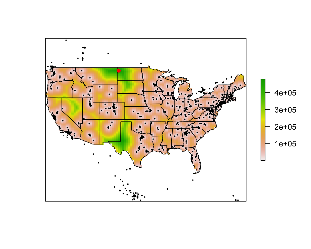
🗑 etc
top
% interactive normal distribution plot, playing around with manipulate function
Manipulate[
Show[
Plot[
PDF[NormalDistribution[\[Mu], \[Sigma]], x],
{x, -10, 10},
AxesOrigin -> {0, 0},
PlotRange -> {-0.1, 0.5},
PlotLabel ->
"\[ScriptCapitalN](" <> ToString[\[Mu]] <> "," <>
ToString[\[Sigma]] <> ")",
PlotStyle -> Directive[Gray, Thickness[0.007]]
],
Plot[
{PDF[NormalDistribution[\[Mu], \[Sigma]], x], 0},
{x, T, 10},
Filling -> 1 -> {2},
FillingStyle -> RGBColor[255/255, 148/255, 112/255, 0.8],
PlotRange -> {-0.1, 0.5},
PlotStyle -> None
]
],
{{\[Mu], 0., Dynamic["\[Mu]=" <> ToString[\[Mu]]]}, -10., 10., 0.2},
{{\[Sigma], 1., Dynamic["\[Sigma]=" <> ToString[\[Sigma]]]}, 1., 5.,
0.1},
{{T, \[Mu], Dynamic["T=" <> ToString[T]]}, \[Mu] - 2.5*\[Sigma],
2.5*\[Sigma] + \[Mu], 0.1},
Delimiter,
Item[Dynamic[Style["p-value=" <> ToString[Round[
NIntegrate[
PDF[NormalDistribution[\[Mu], \[Sigma]], x] // Evaluate, {x,
T, Infinity}]
, 0.001]], FontSize -> 15]], Alignment -> Center]
]
% diversity in math logo made in mathematica!
% just a mobius strip with fancy colors...
x[r_, \[Theta]_] := (1 + r/2 Cos[\[Theta]/2]) Cos[\[Theta]]
y[r_, \[Theta]_] := (1 + r/2 Cos[\[Theta]/2]) Sin[\[Theta]]
z[r_, \[Theta]_] := (r/2 Sin[\[Theta]/2])
ParametricPlot3D[
{
x[r, \[Theta]],
-y[r, \[Theta]],
0.75*z[r, \[Theta]]
},
{r, -1, 1}, {\[Theta], 0, 2 \[Pi]},
PlotStyle -> Red, Mesh -> {10, 1}, MeshStyle -> Black,
MeshShading -> {RGBColor["#CE0000"], RGBColor["#FF0000"],
RGBColor["#FF5252"]}, MeshFunctions -> {#5 &}, Boxed -> False,
Axes -> False, Background -> Black
]